Expression Details
- An expression must be a number, a data column, an appropriately formatted function, or a combination of these items: [5, “X”, sin(“X”), 5sin(“X”)]
- Column names must be entered with quotes. [sin(“X”), “Y”, or abs(“Z”)]
- Supported operators are + – * / ^ ( )
- Functions must contain their arguments in parentheses. [abs(“X”) or sqrt(2)]
- Multiplication can be explicit or implied. [5*“X”, 5“X”, or 5(“X”)]
- Constants must be entered as numbers. Variable parameters (e.g., A, B, C) are not supported.
- Trigonometric functions are evaluated in radians.
- Functions can be nested as long as the proper format is used. [sqrt(abs(“X”))]
Function Syntax
Analysis Functions
| Function | Syntax | Description |
|---|---|---|
| analysis | analysis(“X”,startRow,endRow)
analysis(“X”,2,4) |
Aggregates data from the specified rows of a column named ‘X’ (from all data sets) into a single column of data. |
| dataSets | dataSets(“X”,startRow,endRow)
dataSets(“X”,2,4) |
Creates a column where the row values are the data set names from which the aggregated data was acquired. |
Analysis functions aggregate data from multiple datasets into a single column.
● X—the name of the column from which data is to be copied
● startRow—first row from which data is to be copied
● endRow—last row from which data is to be copied
Blood Pressure Functions
| Function | Syntax | Description |
|---|---|---|
| diastolic | diastolic(“Pressure”,”Time”) | The measured arterial pressure when the heart is at rest. |
| meanArterialPressure | meanArterialPressure(“Pressure”,”Time”) | The pressure value at the max peak used for calculating blood pressure. |
| oscillations | oscillations(“Pressure”,”Time”) | Oscillations of the peaks and valleys used for calculating blood pressure. |
| oscillatoryPeaks | oscillatoryPeaks(“Pressure”,”Time”) | Relative maximum values from the oscillations data used to calculate systolic, diastolic, and pulse values. |
| pulse | pulse(“Pressure”,”Time”) | Pulse rate calculated using the blood pressure sensor inputs. |
| systolic | systolic(“Pressure”,”Time”) | The measured arterial pressure when the heart contracts. |
“Pressure” and “Time” are columns from data collection with a Blood Pressure Sensor (
Boolean Expressions
| Operator | Syntax | Description | Examples |
|---|---|---|---|
| AND | “X” AND “Y” | True (1) if BOTH inputs are True, otherwise False (0). | 1 AND 1 = 1 1 AND 0 = 0 0 AND 1 = 0 0 AND 0 = 0 |
| NOT (!) | ! “X” | True (1) if the input is False. False (0) if the input is True. | ! 1 = 0 ! 0 = 1 |
| OR | “X” OR “Y” | True (1) if AT LEAST one input is True, otherwise False (0). | 1 OR 1 = 1 1 OR 0 = 1 0 OR 1 = 1 0 OR 0 = 0 |
| XOR | “X” XOR “Y” | Exclusive OR True (1) if ONLY one input is True, otherwise False (0). |
1 XOR 1 = 0 1 XOR 0 = 1 0 XOR 1 = 1 0 XOR 0 = 0 |
A Boolean expression is either True (1) or False (0) based on the operator and value of the inputs. When the inputs are columns, the output is a column where Boolean values are determined row-by-row.
- Input value = False (0) when the input is…
⚬ a number = 0 (must identically equal zero, not just round to zero) - Input value = True (1) when the input is…
⚬ any number ≠ 0
⚬ Any non-numeric value (including text string = 0)
⚬ Empty column cells
Operators can be combined (e.g., “X” AND ! “Y”, ! “X” OR “Y”, and ! “X” XOR ! “Y” are valid expressions).
Calculus Functions
| Function | Syntax | Description |
|---|---|---|
| firstDerivative | firstDerivative(“Y”,“X”,numberOfPoints)
firstDerivative(“Position”,“Time”) |
Finds the first derivative of data in column ‘Y’ with respect to column ‘X’. ‘numberOfPoints‘ is set in Session Preferences or can be explicitly set. Default = 7 |
| integral | integral(“Y”, “X”) | Numerical integral – the running sum of the areas of rectangles calculated using the midpoint rule. The ith rectangle is identified by [Yi – Y(i-1)] and [Xi – X(i-1)] |
| secondDerivative | secondDerivative(“Y”,“X”,numberOfPoints)
secondDerivative(“Position”,“Time”) |
Finds the second derivative of data in column ‘Y’ with respect to column ‘X’. ‘numberOfPoints‘ is set in Session Preferences or can be explicitly set. Default = 7 |
Derivative and Integral function parameters:
● Y—a column of data you want to differentiate or integrate
● X—the independent variable column for your data; typically Time
● numberOfPoints—[closest] odd integer ≥ 3 (Session Preference options: 3 ,5, 7, 9, 11, 15, or 21)
For more information on derivative calculations, see How do Logger Pro, Graphical Analysis, LabQuest app, and Vernier Video Analysis calculate velocity and acceleration?
Collapse Functions
| Function | Syntax | Description |
|---|---|---|
| collapse | collapse(“X”) | Creates a new column equivalent to column ‘X’ with the blank cells removed. |
| collapseIndirect | collapseIndirect(“X”,”Y”) | Creates a new column containing values from only the rows in column ‘X’ that correspond to the rows in column ‘Y’ that are numbers (skipping rows where column ‘Y’ has blank cells). |
Collapse functions are used to remove empty cells from columns and to retain correlations between data from other columns (that do not include empty cells). This is helpful when wanting to use functions such as delta() and sum() with columns that contain empty cells.
Column-Fill Functions
| Function | Syntax | Description |
|---|---|---|
| constant | constant(constant,count) | This function generates a column with every cell value = ‘constant’. |
| randInt | randInt(min,max,count) | This function generates a column of random integers between the values of ‘min’ and ‘max’ (inclusive). |
| randReal | randReal(min,max,count) | This function generates a column of random real numbers between the values of ‘min’ and ‘max’ (inclusive). |
| rowNumber | rowNumber() | This function generates a column of values where the cell value is the row number of the cell. (This function has no arguments.) |
| step | step(start,increment,count, firstRow,skip) | Generates a column having ‘count’ rows. The first reported value is ‘start’ and subsequent values are increased or decreased by the value of the ‘increment’. ‘firstRow’ defines the row in which the first value is reported. ‘skip’ defines is the number of rows skipped between reported values. |
| stepColumnBased | stepColumnBased(“X”,start, increment,firstRow,skip) | This function is similar to the step function, except output values will appear only in non-empty rows in column ‘X’. ‘firstRow’ = 2 corresponds to the second non-empty row of column ‘X’. ‘skip’ = 1 will report output values in every other non-empty row of column ‘X’. |
- The data table needs to have active rows in the data set for the fill-value functions to work. These functions do not create active rows automatically.
- The number of rows in the output column is determined by the value of ‘count‘; however, the value is limited by the number of active rows in the dataset.
- When ‘count‘ is a column (e.g., ‘X’), the value of ‘count‘ is number of rows in column ‘X’.
Column-Manipulation Functions
| Function | Syntax | Description |
|---|---|---|
| abs | abs(arg1) | absolute value (|x|) |
| delta | delta(“X”) | The difference between consecutive values from column ‘X’. (The ith value of the output is ith value of ‘X’ minus the (i-1)th value of ‘X’.) The output will have an empty first row. |
| interpolate | interpolate(“Y”,”X”) | This function generates a column where missing values in the ‘Y’ column are filled in using linear interpolation. Column ‘X’ is the independent variable, typically Time. |
| rms | rms(“X”) | Cumulative Root Mean Square of the values in column ‘X’ up to the current row. The output value reported for row 3 is sqrt((X12+X22+X32)/3)) |
| subset | subset(“X”,start,step) | Returns a column of data extracted from column ‘X’ starting with the row numbered ‘start’, incremented by ‘step’ rows. Rows in column ‘X’ that are skipped are blank in the output column. |
| sum | sum(“X”) | The sum of the values in column ‘X’ up to the current row. The output value reported for row 3 is the sum of the column ‘X’ values from rows 1, 2 and 3. |
| value | value(offset,”X”) | Creates a new column based on column ‘X’ by extracting values from column ‘X’ that are ‘offset’ rows from the current row. offset = -2 has column ‘X’ row 1 copied to output row 3 with the first two rows of the output blank. offset = 2 has column ‘X’ row 3 copied to output row 1 with the last two rows of the output blank. offset = 0 will have an output that duplicates column ‘X’. |
Function parameters:
● X and Y—are columns of data
● arg1—can be a number, an expression that resolves to a number, or a column of numbers (“X”).
● offset, start, and step—are integers
Digital Filter Functions
| Function | Syntax | Description |
|---|---|---|
| bandPassFilter | bandPassFilter(“Y”,“X”,bandPassRipple, lowCutoff,highCutoff)
bandPassFilter(“Signal”,“Time”,0.5,1, 50) |
Filter data that have unwanted FFT frequencies outside two ‘cutoff’ values. For EKG/EMG data, filter frequencies below 1 Hz to remove noise from arm or leg movements, and filter frequencies above 50 hz to remove noise from a US power supply. |
| bandStopFilter | bandStopFilter(“Y”,“X”,bandPassRipple, lowCutoff,highCutoff)
bandStopFilter(“Potential”,“Time”,0.5,50,70) |
Filter data that have unwanted FFT frequencies between two ‘cutoff’ values. For voltage data, use a 50 to 70 Hz band stop filter to remove noise from a US power supply. |
| highPassFilter | highPassFilter(“Y”,“X”,bandPassRipple,cutoff)
highPassFilter(“Signal”,“Time”,0,1) |
Filter data that have unwanted FFT frequencies below the ‘cutoff’ value. For EMG data, use a 1 Hz high pass filter to remove noise from muscle movements such as a twitch. |
| lowPassFilter | lowPassFilter(“Y”,“X”,bandPassRipple,cutoff)
lowPassFilter(“Signal”,“Time”,0,50) |
Filter data that have unwanted FFT frequencies above the ‘cutoff’ value. For EKG data, use a 50 Hz low pass filter to remove noise from a power supply affecting your data. |
| timeDecayFilter | timeDecayFilter(“Y”,“X”,timeDecay) | Use this function to apply a time decay to the data. |
Digital Filter functions are designed to work with analog sensors and/or truly analog signals. Signals or sensors that perform digital signal processing may not work well with these features.
- Y—the column of data to which the filter is being applied
- X—the independent variable column for your data; typically Time
- bandPassRipple—This value is the percentage of pass-band
⚬ Low Pass and High Pass filters are typically 0, which applies a Butterworth filter
⚬ Band Stop and Band Pass filters are typically 0.5, which applies a Chebyshev filter
⚬ To mimic an analog filter circuit, set the bandPassRipple to 0
⚬ In most cases, a bandPassRipple set to 0.1 will give the best results - cutoff, lowCutoff, highCutoff—the FFT frequency cutoff value used for the filter; must be a number
- timeDecay—time decay constant, typically in seconds
Energy Sensor Functions
| Function | Syntax | Description |
|---|---|---|
| energy | energy(“Potential”,”Current”) | Calculates Energy in Joules (J) |
| power | power(“Potential”,”Current”) | Calculates Power in milliwatts (mW) |
| resistance | resistance(“Potential”,”Current”) | Calculates Resistance in ohms (Ω) |
“Potential” (measured in V) and “Current” (measured in mA) are columns from data collection with a Vernier Energy Sensor (
Exponential and Logarithmic Functions
| Function | Syntax | Description | Examples |
|---|---|---|---|
| exp | exp(arg1) | Natural (base-e) exponential function (ex) | exp(2) ≈ 7.389 |
| exp2 | exp2(arg1) | base-2 exponential function (2x) | exp2(2) = 4 |
| expm1 | expm1(arg1) | ex–1 or exp(x)–1 Greater accuracy for ‘x’ values close to 0. Inverse of log1p(x). |
expm1(0.005) ≈ 0.005012521 |
| ln | ln(arg1) | Natural or base-e logarithmic function (ln x or loge x) |
ln(2.719) ≈ 1 |
| log | log(arg1) | common or base-10 logarithmic function (log x or log10x) |
log(1000) = 3 |
| log1p | log1p(arg1) | ln(1+x) Greater accuracy for ‘x’ values close to 0. Inverse of expm1(x) |
log1p(0.005012512) ≈ 0.005 |
| log2 | log2(arg1) | base-2 logarithmic function (log2x) | log2(8) = 3 |
● arg1—can be a number, an expression that resolves to a number, or a column of numbers (“X”).
Modulo (Integer Remainder) Functions
| Function | Syntax | Description | Examples |
|---|---|---|---|
| mod | mod(arg1,arg2) | Modulo – integer remainder of X/Y mod(x,y) = x – y*trunc(x/y) |
mod(5,4) = 1 mod(6,4) = 2 mod(7,4) = 3 |
| remainder | remainder(arg1,arg2) | ISEE – integer remainder of X/Y remainder(x,y) = x – y*round(x/y) |
remainder(5,4) = 1 remainder(6,4) = -2 remainder(7,4) = -1 |
● arg1—can be a number, an expression that resolves to a number, or a column of numbers (“X”).
Photogate and Projectile Launcher Functions
Use these functions to calculate typical photogate measurements when collecting time-based data.
Power Functions (xn)
| Function | Syntax | Description | Examples |
|---|---|---|---|
| cbrt | cbrt(arg1) | cube root | cbrt(27) = 3 |
| pow | pow(arg1,arg2) | power (xy) x = arg1 and y = arg2 |
pow(5,3) = 125 power(3,5) = 243 |
| sqrt | sqrt(arg1) | square root | sqrt(81) = 9 |
● arg1—can be a number, an expression that resolves to a number, or a column of numbers (“X”).
Rate and Beats Per Minute Functions
| Function | Syntax | Description |
|---|---|---|
| rate | rate(“Y”,”X”,t,m1,m2,n,dt)
rate(“Signal”,”Time”,15,0.4,0.6,0,5) |
The rate of column ‘Y’ with respect to column ‘X’, where t is the time interval measured, ‘m1’ is min percentage threshold, ‘m2’ is max percentage threshold, ‘n’ is noise threshold, and ‘dt’ is the offset to start of the next range. |
| beatsPerMinute | beatsPerMinute(“Y”,”X”,t,m1,m2,n,dt) | This function is similar to the rate function except that the interval (‘t’) is in seconds and the output values are in minutes. If column ‘X’ is in seconds, then beatsPerMinute(“Y”,”X”) = 60*rate(“Y”,”X”) |
● Y—a column of data for which you want to determine the rate of oscillation
● X—the independent variable column for your data; typically Time
Rounding Functions
| Function | Syntax | Description | Examples |
|---|---|---|---|
| ceiling | ceiling(arg1) | Nearest integer greater than a given number. | ceiling(3.5) = 4 ceiling(-3.5) = -3 |
| floor | floor(arg1) | Nearest integer less than a given number. | floor(3.5) = 3 floor(-3.5) = -4 |
| integer | integer(arg1) | Integer part of a given number. interger(arg1) = trunc(arg1) |
interger(3.5) = 3 interger(-3.5) = -3 |
| round | round(arg1) | Rounds to the nearest integer. When the decimal value of ‘arg1’ is exactly 0.5, values are rounded up if ‘arg1’>0 and rounded down if ‘arg1′<0. |
round(3.5) = 4 round(-3.5) = -4 |
| trunc | trunc(arg1) | Truncate – Integer part of a given number. trunc(arg1) = interger(arg1) |
trunc(3.5) = 3 trunc(-3.5) = -3 |
● arg1—can be a number, an expression that resolves to a number, or a column of numbers (“X”).
Smoothing Functions
| Function | Syntax | Description |
|---|---|---|
| smoothAve | smoothAve(“Y”) | This function returns a column of moving averages of the values in column ‘Y’. ‘numberOfPoints’ is set in Session Preferences. Default = 7 |
| smoothSG | smoothSG(“Y”,”X”,numberOfPoints)
smoothSG(“Position”,“Time”) |
Savitsky-Goley smoothing fits a polynomial to a number of points around each point and computes the value of the polynomial at that point. ‘numberOfPoints’ is set in Session Preferences or can be explicitly set. Default = 7 |
Smoothing functions.
● Y—is the columns of numbers you want to smooth
● X—the independent variable column for your data; typically Time
● numberOfPoints—[closest] odd integer ≥ 3 (Session Preferences: 3 ,5, 7, 9, 11, 15, or 21.)
Statistical Functions
| Function | Syntax | Description |
|---|---|---|
| max | max(“X”) | Reports the largest number in column ‘X’. |
| max2 | max2(“X”,”Y”) max2(“X”, 5) |
Compares the values in column ‘X’, row by row, with values in column ‘Y’ (or some constant) and reports the larger of the two numbers for the corresponding row in the output column. |
| mean | mean(“X”) | Arithmetic mean of the numbers in column ‘X’. |
| median | median(“X”) | The median (middle) value of the ranked (ordered) values in column ‘X’. Column ‘X’ does not need to be sorted. |
| min | min(“X”) | Reports the smallest number in column ‘X’. |
| min2 | min2(“X”,”Y”) min2(“X”,5) |
Compares the values in column ‘X’, row by row, with values in column ‘Y’ (or some constant) and reports the smaller of the two numbers for the corresponding row in the output column. |
| numRows | numRows(“X”) | This outputs the number of rows in column ‘X’. |
| rms | rms(“X”) | Cumulative Root Mean Square of the values in column ‘X’ up to the current row. The output value reported for row 3 is sqrt((X12+X22+X32)/3)) |
| stddev | stddev (“X”) | The standard deviation of the numbers in a column ‘X’. |
● X and Y—are columns of numbers
● arg1—can be a number, an expression that resolves to a number, or a column of numbers (“X”).
Trigonometric Functions
● Trigonometric functions are evaluated in radians.
Miscellaneous Functions
| Function | Syntax | Description | Examples |
|---|---|---|---|
| copysign | copysign(arg1,arg2) | Changes the sign of a number to match the sign of another number | copysign(-5,1)=5 copysign(5,-2)=-5 |
| dim | dim(arg1,arg2) | Calculates the difference between two numbers and reports the value if the difference is ≥ 0; otherwise reports 0. | dim(10,8) = 2 dim(10,9.9) = 0.1 dim(8,10) = 0 |
| erf | erf(arg1) | error function or Gauss error function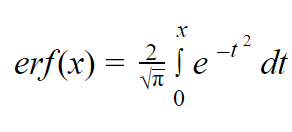 |
erf(.25) ≈ 0.276 |
| erfc | erfc(arg1) | Complementary error function erfc(x) = 1 – erf(x) |
erfc(.25) ≈ 0.724 |
| hypot | hypot(arg1,arg2) | Hypotenuse hypot(x,y) = sqrt(x2 + y2) |
hypot(5,12) = 13 hypot(4,3) = 5 |
| logb | logb(arg1) | floating-point base logarithmic function, logb(x), returns the unbiased exponent value of ‘x‘ as a signed integer represented as a floating-point value. logb(arg1) = floor(log2(abs(arg1))) |
logb(10) = 3 logb(-1.5) = 0 logb(0.1) = -4 |
| nextafter | nextafter(arg1,arg2) | Computes next representable float after X in the direction of Y | nextafter(1/0,1)=infinity |
| PolarRadius | PolarRadius(arg1,arg2) | Finds r when coverting cartesian to polar coordinates (x,y) → (r,θ) r = sqrt(x2 + y2) = hypot(x,y) |
PolarRadius(1,1)≈1.414 |
| PolarTheta | PolarTheta(arg1,arg2) | Finds θ when coverting cartesian to polar coordinates (x,y) → (r,θ) θ = atan(y/x); 0 ≤ θ < 2π radians |
PolarTheta(1,1)≈0.785 |
● arg1—can be a number, an expression that resolves to a number, or a column of numbers (“X”).